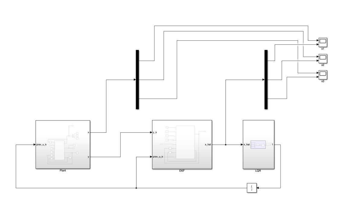
Setting up an optical communication link between underwater robots is tough due to severe signal attenuation and the need for precise alignment. For this project, my partner and I worked to recreate and verify an advanced control framework using a recursive Extended Kalman Filter (EKF) and a Linear Quadratic Regulator (LQR). We engineered the simulation using custom blocks in MATLAB and Simulink.
You can find the codebase and detailed report with all calculations on GitHub.
EKF & LQR Implementation
Instead of relying on prebuilt Simulink blocks, which weren’t robust enough for this specific setup, we wrote custom MATLAB function blocks for both the plant and the controllers.
Standalone EKF & LQR Testing
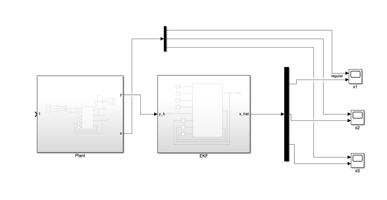
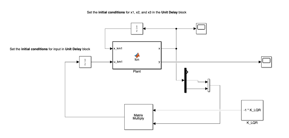
Following the Principle of Separation, we built and tested the EKF and LQR completely independently before attempting to close the loop.
Standalone EKF Tracking
The state estimator runs a recursive predict-update cycle, propagating the state and error covariance ahead, computing the optimal Kalman gain from incoming measurements, and updating the estimated states:
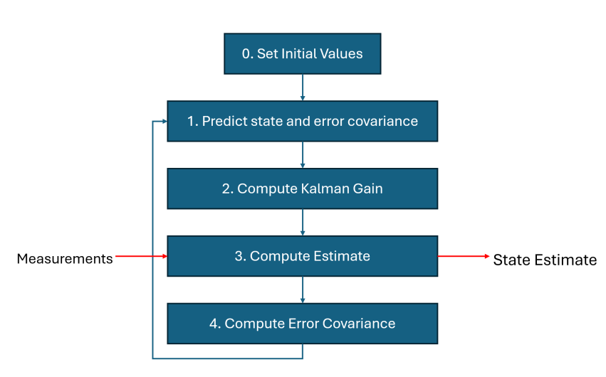
Recursive Extended Kalman Filter cycle: initializing state priors, predicting state and covariance, computing the Kalman gain, incorporating incoming measurements to update the state estimate, and propagating error covariance to the next time step.
The standalone EKF successfully filtered the Gaussian measurement noise and locked onto the true system values after about two seconds of simulation time:
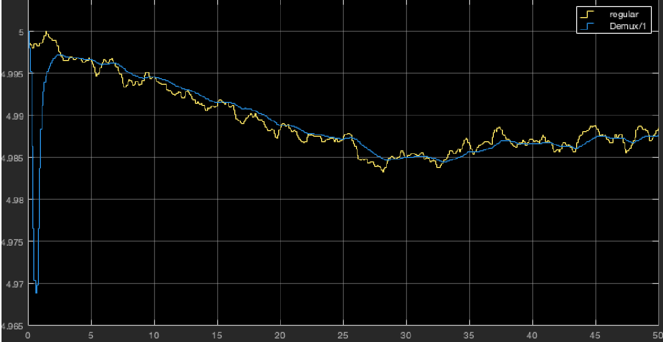
State x1 tracking: received optical power (P_rx) estimate converges rapidly to the true value despite simulated Gaussian noise.
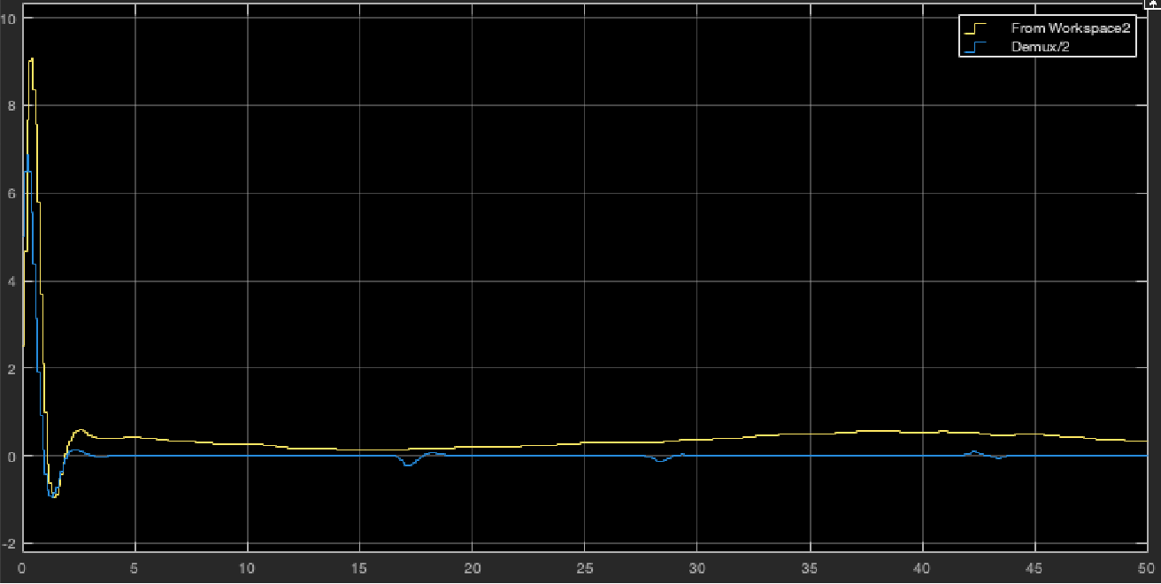
State x2 tracking: receiver orientation error (θ) estimate smoothly tracks and locks onto the true state within two seconds.
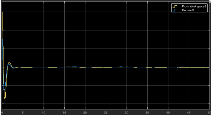
State x3 tracking: actuator angular velocity (θ_dot) estimate successfully reconstructed by the EKF from sequential measurements.
Standalone LQR Regulation
Running on its own with the known true states, the LQR controller successfully drove the initial angular displacement and angular velocity back to zero within 20 time steps (approximately two seconds):
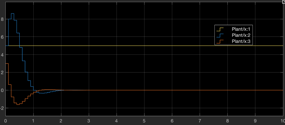
Standalone LQR response: the controller drives orientation error (x2, blue) and angular velocity (x3, orange) smoothly to zero from initial perturbation, while optical power (x1, yellow) remains stable.
Closed-Loop Troubleshooting & Takeaways
While the EKF and LQR worked perfectly on their own, the fully closed-loop system failed to stabilize. The estimated states diverged, and the controller couldn’t drive the orientation back to zero. We ran through a series of systematic troubleshooting steps to isolate the issue:
- Adding the $\psi_k$ Offset: We tried adding the artificial angle offset term ($\psi_k$) used in the original reference paper’s state estimation, but it actually worsened the results and introduced more oscillation.
- Covariance Tuning: We tuned the $Q_{EKF}$, $R_{EKF}$, and $Q_{LQR}$ parameters. This changed the filter’s behavior but didn’t solve the instability or yield a demonstrable improvement.
- Actuator Limits: We bounded the state values, limiting the angle to $\pm 15$ degrees and 0.2 degrees per timestep. This slowed the response but still ultimately ended in oscillation.
- Timesteps & Initial Conditions: Adjusting the simulation timestep just stretched or compressed the response, and changing initial conditions offered no improvement.
Final Thoughts
This project was a great lesson in the reality of control systems. According to the Principle of Separation, independent estimators and controllers should combine perfectly. In practice, a hidden modeling flaw in the nonlinear plant or a missing theoretical constraint can easily break the closed loop.